



- connectivity: multi-resolution landscape connectivity in Python
The eco-connectivity Python package implements an efficient multi-resolution least-cost algorithm for calculating connectivity-based biodiversity indicators, including Connected Habitat (connectivity-adjusted condition), the Protected Area Connectedness Index (PARC-connectedness), and the Bioclimatic Ecosystem Resilience Index (BERI). It combines habitat condition, least-cost paths and dispersal kernels to estimate how much surrounding habitat is accessible across dispersal scales. The algorithm retains fine spatial resolution near each focal cell and progressively coarsens with distance, enabling analysis of large landscapes. PARC-connectedness incorporates protected-area coverage, while BERI uses current and future climate-related compositional similarity to assess ecosystem resilience under climate change. The package uses rasterio and geopandas for spatial data processing and the connectivity-core Rust engine, shared with the R package connectivity, for numerical computations. See Valavi et al. (2026) for the full method.
The package is published on PyPI as eco-connectivity (NOTE: pip install connectivity installs an unrelated package):
pip install eco-connectivityThe import name is still connectivity:
from connectivity import connectedness, beriTo build the latest development version from the GitHub repository, install Rust first, then run:
git clone https://github.com/csiro/connectivity.git
cd connectivity
pip install ./pythonThe numerical engine is a separate Rust crate, connectivity-core, which works on in-memory arrays without Python, GDAL or file I/O. Rust programs can use it directly; see its README and crate documentation. cargo test --workspace runs every Rust test, and cargo test -p connectivity-core needs no Python.
Resolve the bundled example paths once so they can be reused throughout the analysis:
from connectivity import beri, connectedness, example_data_path, resolution_info

condition_file = example_data_path("site_condition")
pa_file = example_data_path("pa_proportion")
current_file = example_data_path("transgrids/1990")
future_files = [
    example_data_path("transgrids/IPS50_45"),
    example_data_path("transgrids/GFD50_85"),
]
To bound the spatial extent of the connectivity calculation, the algorithm limits how far it searches across neighboring cells in the condition raster. The approximate one-sided search reach is computed as:
max_reach = outer_window * max(levels) * resolution. For example, with a 1 km resolution raster, a max-level of 32, and an outer_window of 11, the resulting search reach is:
distance = outer_window × max_level × resolution
         = 11 × 32 × 1 km
         = 352 km
Use resolution_info() to preview how candidate levels will change raster
dimensions and approximate search reach before running the analysis:
resolution_info(condition_file, outer_window=9)File: .../connectivity/data/site_condition.tif
Base raster: 588 x 516 cells (303.41K total)
Base resolution: 0.008333 degrees
CRS: EPSG:4326
Bands: 1
Data type(s): float32
Nodata: -9999.0
Outer window: 9
Small-dimension warning threshold: < 16 cells
Distance note: approximate km values use centre latitude -41.550
Candidate internally generated levels:
Level Width Height Cells % base Resolution Reach Reach km Note
1 588 516 303.41K 100.000% 0.008333 degrees 0.075 degrees 8.349 km
2 294 258 75.85K 25.000% 0.01667 degrees 0.15 degrees 16.7 km
4 147 129 18.96K 6.250% 0.03333 degrees 0.3 degrees 33.4 km
8 74 65 4.81K 1.585% 0.06667 degrees 0.6 degrees 66.79 km
16 37 33 1.22K 0.402% 0.1333 degrees 1.2 degrees 133.6 km
32 19 17 323 0.106% 0.2667 degrees 2.4 degrees 267.2 km
64 10 9 90 0.030% 0.5333 degrees 4.8 degrees 534.3 km small grid; review
128 5 5 25 0.008% 1.067 degrees 9.6 degrees 1.07K km small grid; review
256 3 3 9 0.003% 2.133 degrees 19.2 degrees 2.14K km small grid; review
512 2 2 4 0.001% 4.267 degrees 38.4 degrees 4.27K km small grid; review
The default window_mode="circular" uses source-centered circular annuli with
fractional area/count support at annulus boundaries. The
window_mode="square" option uses the same source-centered fractional
construction with square annuli. These modes change indicator values, so
compare outputs only between runs that use the same window mode.
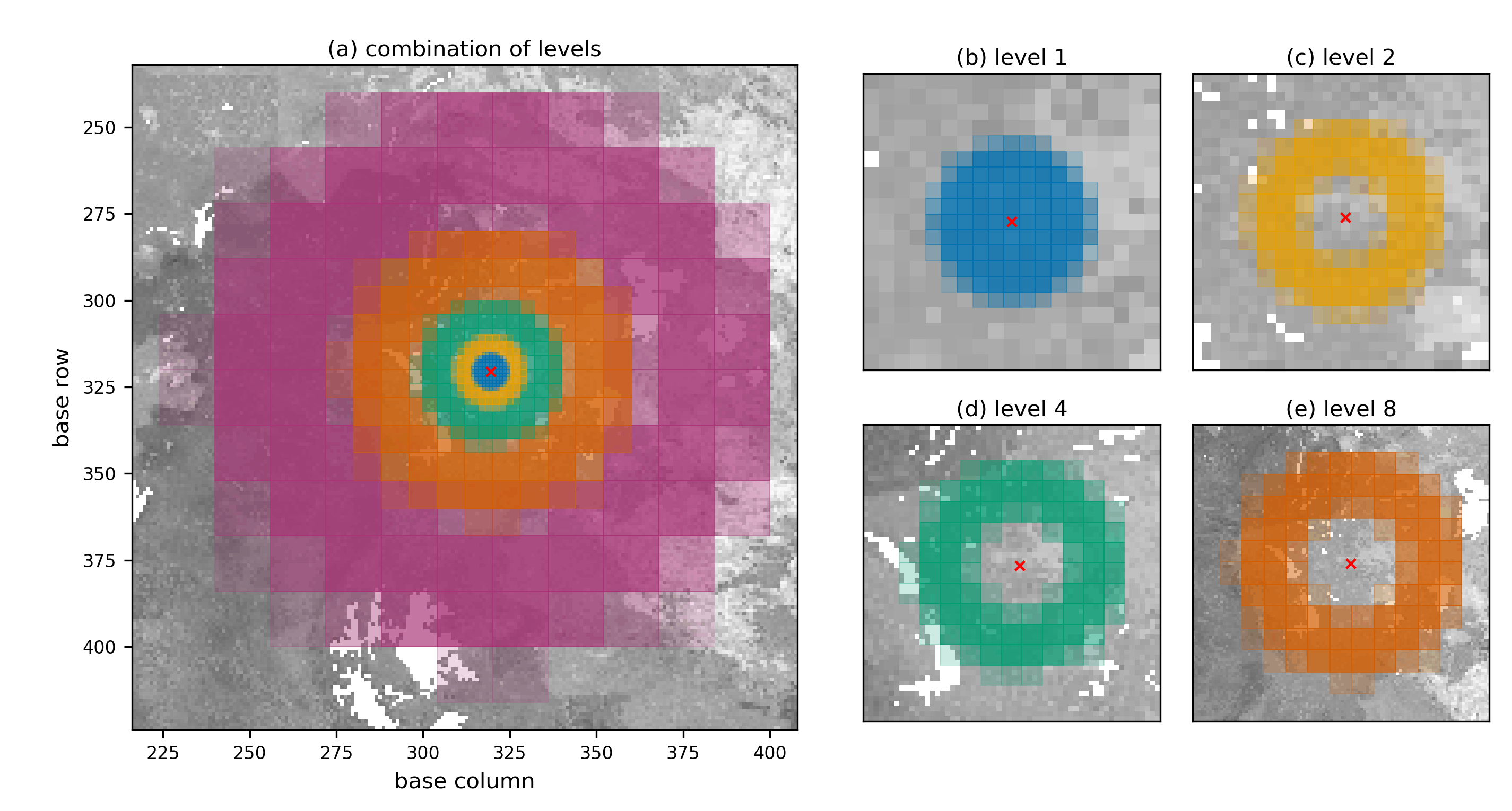
Each coloured neighbourhood represents a different raster aggregation level. Fine levels capture nearby cells at higher resolution, while coarser levels extend the search over larger distances. Their contributions are combined into a single graph, in which the least-cost path from the focal cell is calculated for each aggregated cell. See Valavi et al. (2026) for the full method.
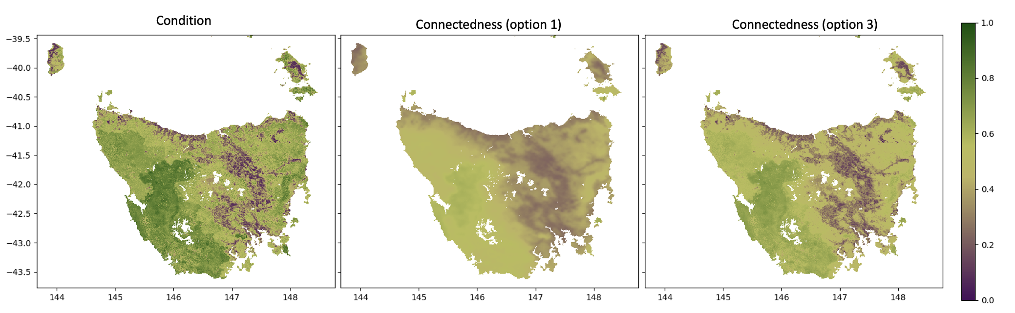
To compute connected-habitat (or plain connectedness), you only need a habitat condition raster. Use option argument to generate the connected-habitat from connectedness and input condition with:
connectednessconnectedness * conditionsqrt(connectedness * condition)— geometric mean (default)
connd = connectedness(
    condition_file = condition_file,
    lambdas = [2, 20, 200],
    max_cost = 2.0,
    window_size = 5,
    outer_window = 11,
    window_mode = "circular",
    levels = [2, 4, 8, 16, 32],
    option = 3,
    filename = "./results/connected_habitat.tif"
)
By default the habitat condition raster does double duty: it weights how costly each cell is to
move through and supplies the habitat value used in the indicator. Pass an optional
resistance_file to decouple these two roles. The resistance raster (values in [0, 1],
higher = harder to cross, scaled with resistance_scale) then drives only the least-cost path
traversal, while condition still supplies the habitat value:
connd = connectedness(
    condition_file = condition_file,
    resistance_file = resistance_file,   # optional; decoupled movement-cost surface
    resistance_scale = None,             # divide resistance into [0, 1] if needed
    max_cost = 2.0,
    window_mode = "circular",
    levels = [2, 4, 8, 16, 32],
)
The edge weight becomes w = (1.0 - max_cost) * (1 - resistance) + max_cost, so resistance = 0
is free (w = 1) and resistance = 1 is the most costly (w = max_cost). When resistance_file
is omitted, condition is used for traversal as before, and the output is unchanged. Cells valid in
condition but missing a resistance value fall back to condition for traversal and raise a warning,
so the analysis domain is never changed silently. The same resistance_file / resistance_scale
arguments are available on beri().
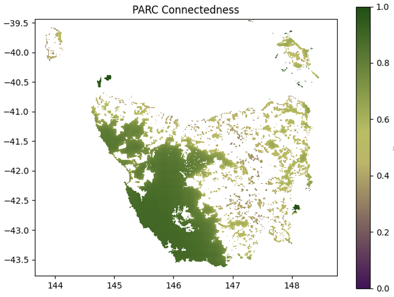
To compute PARC-connectedness, provide both:
- a habitat condition raster, and
- a protected-areas proportion raster.
When pa_file (proportion of protected-areas in each cell) is supplied, the function automatically returns PARC-connectedness instead of standard connectedness.
parcc = connectedness(
    condition_file = condition_file,
    pa_file = pa_file,
    lambdas = [2, 20, 200],
    max_cost = 2.0,
    window_size = 5,
    outer_window = 11,
    window_mode = "circular",
    levels = [2, 4, 8, 16, 32],
    filename = "./results/parc_connectedness.tif"
)
Use pixel_coverage() when you need the proportion of each raster pixel covered
by polygon geometry. The calculation is backed by a performant Rust
implementation:
from connectivity import pixel_coverage

coverage = pixel_coverage(
    "./data/polygons.gpkg",
    condition_file,
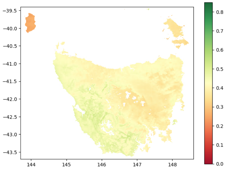
)To compute BERI, you must provide:
- a condition raster
- current GDM transgrids
- one or more future transgrids scenarios (as a list)
beris = beri(
    condition_file = condition_file,
    current_file = current_file,
    future_files = future_files,
    lambdas = [2, 20, 200],
    max_cost = 2.0,
    window_size = 5,
    outer_window = 11,
    window_mode = "circular",
    levels = [2, 4, 8, 16, 32],
    filename = "./results/berri.tif"
)
To run the model using tiles, create a rectangular tile polygon as a GeoDataFrame
and pass it to the polygon_mask argument. This limits data loading to only the
portion required for the tile, i.e. the output core plus the internally buffered
neighborhood.
Use make_tile() to generate non-overlapping output-core tiles whose internal
boundaries align with the coarsest aggregation level. This is preferred over
creating overlap-expanded tile polygons externally. Be sure to set
closed_border = False (the default) so that neighborhood information is
included around each tile core.
from connectivity import connectedness, make_tile

levels = [2, 4, 8, 16, 32]

tile_id = 0
tile_poly = make_tile(
    raster_file = condition_file,
    nrows = 4,
    ncols = 4,
    tile_id = tile_id,
    align_to = max(levels),
)

connd = connectedness(
    condition_file = condition_file,
    polygon_mask = tile_poly,
    closed_border = False,
    margin_px = 32,
    lambdas = [2, 20, 200],
    max_cost = 2.0,
    window_size = 5,
    outer_window = 11,
    window_mode = "circular",
    levels = levels,
    option = 1,
    filename = f"./results/connected_habitat_tile_{tile_id}.tif"
)
For large, uneven workloads, use balanced tiles:
tile_poly = make_tile(
    raster_file = condition_file,
    nrows = 4,
    ncols = 4,
    tile_id = tile_id,
    align_to = max(levels),
    balanced = True,
    io_weight = 0.1,
)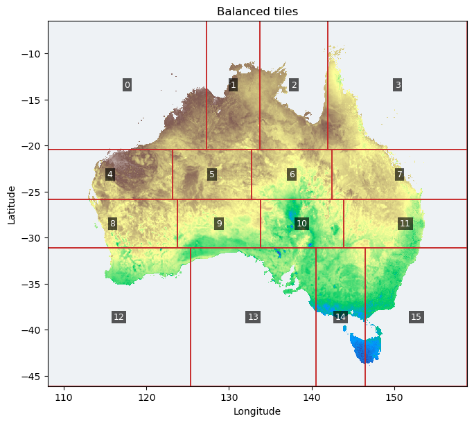
Balanced tiling uses a deterministic raster-mask cost estimate while preserving
the same align_to boundary alignment. It is useful for global rasters where
some tiles contain mostly ocean or nodata and others contain many valid land
pixels. Use balanced = False (the default) when equal aligned tiles are enough.
When balanced = False, io_weight is ignored.
To cite the connectivity library in publications and reports, please use:
Valavi, R., Mokany, K., Ware, C., Vickers, M., Giljohann, K. M., & Ferrier, S. (2026). A scalable multi-resolution framework for connectivity-based biodiversity indicators. EcoEvoRxiv, preprint. doi:10.32942/X2S68V.
Underlying methods:
- Drielsma, M., Ferrier, S., & Manion, G. (2007). A raster-based technique for analysing habitat configuration: The cost–benefit approach. Ecological Modelling, 202(3–4), 324–332. doi:10.1016/j.ecolmodel.2006.10.016.
- Drielsma, M. J., Love, J., Taylor, S., Thapa, R., & Williams, K. J. (2022). General Landscape Connectivity Model (GLCM): a new way to map whole of landscape biodiversity functional connectivity for operational planning and reporting. Ecological Modelling, 465, 109858. doi:10.1016/j.ecolmodel.2021.109858.
- Harwood, T., Love, J., Drielsma, M., Brandon, C., & Ferrier, S. (2022). Staying connected: assessing the capacity of landscapes to retain biodiversity in a changing climate. Landscape Ecology, 37, 3123–3139. doi:10.1007/s10980-022-01534-5.
- Ferrier, S., Harwood, T. D., Ware, C., & Hoskins, A. J. (2020). A globally applicable indicator of the capacity of terrestrial ecosystems to retain biological diversity under climate change: The bioclimatic ecosystem resilience index. Ecological Indicators, 117, 106554. doi:10.1016/j.ecolind.2020.106554.
Developed at the Commonwealth Scientific and Industrial Research Organisation
(CSIRO). Copyright © 2026 CSIRO. The code is distributed under the
MIT licence.
The Python binding uses PyO3/maturin for its interface and rasterio,
geopandas and shapely for its spatial workflows.
The bundled Tasmania data are licensed separately under CC BY-NC-SA 4.0. Please cite:
Ware, C., Valavi, R., Vickers, M., Giljohann, K. M., Mokany, K., Purvis, A., Walkden, P., De Palma, A., Duffin, C., Contu, S., Harwood, T., Hoskins, A., & Ferrier, S. (2026). Global biodiversity indicator data for BHI, BERI, PARC-representativeness, PARC-connectedness and ecosystem condition (2000–2024). Version 4. CSIRO Data Collection. doi:10.25919/3aka-y730.
See the example-data README
for layer metadata and attribution, also installed with the package as
connectivity/data/README.md.